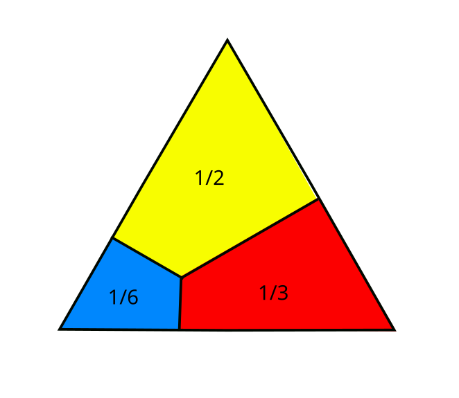
The problem goes: If an equilateral triangle is cut into areas in proportions 1:2:3 by lines perpendicular to the sides, what should be the length of these lines? The following picture shows the proportions of the total area:
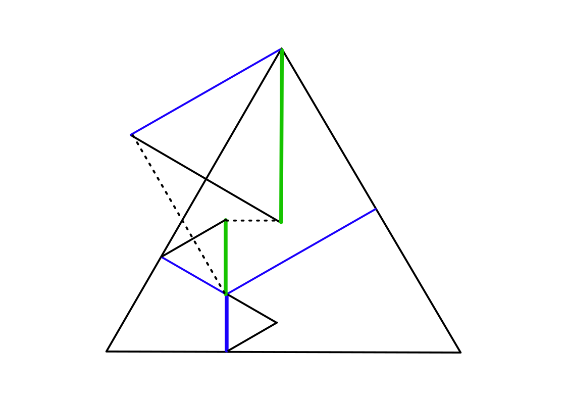
It can be shown that all the lines perpendicular to the sides add up to the length between a corner and the opposite mid-side. One way of doing this is building one equilateral triangle for each of the lines and piling them on top of each other in the middle of the big triangle:
The problem is: given a fixed value of the height of the triangle (we can set it to 1), find the values a, b, c that produce a partition of the triangle's area in 1/6, 1/3 and 1/2. The relevant lengths are shown in the following diagram:
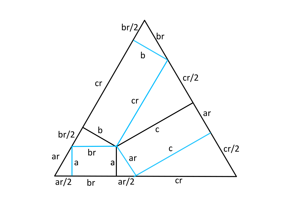
where
\[r = 2/\sqrt{3} \]
. It is easy to verify that the areas are:
\[ A_1 = \frac{r}{4}\left( a^2 + 4ab + b^2 \right) \]
\[ A_2 = \frac{r}{4}\left( a^2 + 4ac + c^2 \right) \]
\[ A_3 = \frac{r}{4}\left( c^2 + 4bc + c^2 \right) \]
We can put these areas as quadratic forms defined by area matrices as follows:
\[\begin{matrix} M_1 = \frac{r}{4}\begin{pmatrix} 1 & 2 & 0 \\ 2 & 1 & 0 \\ 0 & 0 & 0 \end{pmatrix} & M_2 = \frac{r}{4}\begin{pmatrix} 1 & 0 & 2 \\ 0 & 0 & 0 \\ 2 & 0 & 1 \end{pmatrix} & M_3 = \frac{r}{4}\begin{pmatrix} 0 & 0 & 0 \\ 0 & 1 & 2 \\ 0 & 2 & 1 \end{pmatrix} \end{matrix} \]
We have then set of thee quadratic equations (one for $A_1$, one for $A_2$ and one for $A_3$) of which two are independent, and a linear one coming from $a+b+c = 1$. The first step I'll take is to transform variables to make two of the quadratic equations depend on only single-variable square terms, which means diagonal coefficient forms. I'd want to do this with a linear transformation to variables $\begin{pmatrix} x & y & z \end{pmatrix} = \begin{pmatrix} a & b & c \end{pmatrix} T$ where $x + y + z = a + b + c$ (here we multiply by right as we'd do in the matrix representation with a row vector. A column vector, or a vector in the dual space from this, would be multiplied by left).
This can be done with a Household transformation. A Householder transformation $H$ is defined by a vector, which it will leave unchanged but changed sign: $ H_V V= -V$ (for a column vector $V$). $-H$ will, of course, not even change the sign of the vector. Our transformation would be defined by the vector $(1,1,1)$ which represents $a+b+c$
\[ T = -\text{Identity}_{3\times 3} + \frac{2}{3}\begin{pmatrix} 1 \\ 1 \\ 1 \end{pmatrix}\begin{pmatrix} 1 & 1 & 1 \end{pmatrix} = \frac{1}{3}\begin{pmatrix}-1 & 2 & 2 \\ 2 & -1 & 2 \\ 2 & 2 & -1 \end{pmatrix}\]
The transformed matrices will be:
\[\begin{matrix} \tilde{M_1} = \frac{r}{4}\begin{pmatrix} -1 & 2 & 2 \\ 2 & -1 & 2 \\ 2 & 2 & 8 \end{pmatrix} & \tilde{M_2} = \frac{r}{4}\begin{pmatrix} -1 & 2 & 2 \\ 2 & 8 & 2 \\ 2 & 2 & -1 \end{pmatrix} & \tilde{M_3} = \frac{r}{4}\begin{pmatrix} 8 & 2 & 2 \\ 2 & -1 & 2 \\ 2 & 2 & -1 \end{pmatrix} \end{matrix} \]
It is easy to see that some combinations of them will be diagonal, and so we can define the following equations:
\[ A_3 - A1 = \frac{r}{12} \begin{pmatrix} x & y & z \end{pmatrix} \begin{pmatrix} 1 & 0 & 0 \\ 0 & 0 & 0 \\ 0 & 0 & -1 \end{pmatrix} \begin{pmatrix} x \\ y \\ z \end{pmatrix} = \frac{r}{12}\left (z^2 - x^2 \right)\]
\[ A_3 - A2= \frac{r}{23} \begin{pmatrix} x & y & z \end{pmatrix} \begin{pmatrix} 1 & 0 & 0 \\ 0 & -1 & 0 \\ 0 & 0 & 0 \end{pmatrix} \begin{pmatrix} x \\ y \\ z \end{pmatrix} = \frac{r}{12}\left (y^2 - x^2 \right)\]
Putting one varaiable in terms of the other two (e.g. $c = 1-a-b$) will leave us two independent quadratic equations:
\[ A_2 = \frac{r}{4}\left( a^2 + 4a(1-a-b) + (1-a-b)^2 \right) = 1 -2a^2 + 2a - 2b + 2ab + b^2 \]
\[ A_3 = \frac{r}{4}\left( b^2 + 4b(1-a-b) + (1-a-b)^2 \right) = 1 -2b^2 + 2b - 2a + 2ab + a^2 \]
These are a slightly different quadratic forms, which again can be expressed in matrix form:
\[ A_2 = \frac{r}{4} \begin{pmatrix} 1 & a & b \end{pmatrix} \begin{pmatrix} 1 & 1 & -1 \\ 1 & -2 & 1 \\ -1 & 1 & 1 \end{pmatrix} \begin{pmatrix} 1 \\ a \\ b \end{pmatrix} \]
\[ A_3 = \frac{r}{4} \begin{pmatrix} 1 & a & b \end{pmatrix} \begin{pmatrix} 1 & -1 & 1 \\ -1 & 1 & 1 \\ 1 & 1 & -2 \end{pmatrix} \begin{pmatrix} 1 \\ a \\ b \end{pmatrix} \]
This immediately suggests the equation
\[ A_2 + A_3 = \frac{r}{4} \begin{pmatrix} 1 & a & b \end{pmatrix} \begin{pmatrix} 2 & 0 & 0 \\ 0 & -1 & 0 \\ 0 & 0 & -1 \end{pmatrix} \begin{pmatrix} 1 \\ a \\ b \end{pmatrix} \]
\[ A_2 + A_3 = \frac{r}{4}\left( 2 - a^2 - b^2 \right) \]
Each one of these matrices are null in one column and one row, while the other two contain the block $\begin{pmatrix} 1 & 2 \\ 2 & 1 \end{pmatrix}$.
These can be spectrally decomposed as follows:
\[
\begin{pmatrix} 1 & 2 \\ 2 & 1\end{pmatrix} = \frac{3}{2}\begin{pmatrix} 1 \\ 1\end{pmatrix}\begin{pmatrix}1 & 1\end{pmatrix} + -\frac{1}{2}\begin{pmatrix}1 \\ -1 \end{pmatrix}\begin{pmatrix}1 & -1\end{pmatrix}\]
This means that the areas can be written as:
\[ A_1 = \frac{r}{8}\left( 3(a+b)^2 - (a-b)^2\right) \]
\[ A_2 = \frac{r}{8}\left( 3(a+c)^2 - (a-c)^2\right) \]
\[ A_3 = \frac{r}{8}\left( 3(b+c)^2 - (b-c)^2\right) \]
We still have a
So far we have not used the fact that $a+b+c = 1$. We can introduce this by replacing $a+b = 1-c$, $a+c = 1-b$ and $b + c = 1-a$. This means that we have to extend the coefficient matrices to represent linear terms, as follows:
\[ A_1 = \frac{r}{8}\left( 3(1 - 2c + c^2) - (a^2 - 2ab + b^2)^2\right) \]
\[ A_2 = \frac{r}{8}\left( 3(1 - 2b + b^2) - (a^2 - 2ac + c^2)\right) \]
\[ A_3 = \frac{r}{8}\left( 3(1 - 2c + c^2) - (b^2 -2bc + c^2)\right) \]
\[\begin{matrix} M_1 = \frac{r}{4}\begin{pmatrix} 3 & 0 & 0 & 3 \\ 0 & 1 & 2 & 0 \\ 0 & 2 & 1 & 0 \\ 3 & 0 & 0 & 3 \end{pmatrix} & M_2 = \frac{r}{4}\begin{pmatrix} 3 & 0 & 3 & 0 \\ 0 & 1 & 0 & 2 \\ 3 & 0 & 3 & 0 \\ 0 & 2 & 0 & 1 \end{pmatrix} & M_3 = \frac{r}{4}\begin{pmatrix} 3 & 3 & 0 & 0 \\ 3 & 3 & 0 & 0 \\ 0 & 0 & 1 & 2 \\ 0 & 0 & 2 & 1 \end{pmatrix} \end{matrix} \]
This is still not very useful, as solving a system of three entangled quadratic equations would entail solving a six degree equation. A symmetrical variable transformation is likely to produce a more convenient set of equations:
\[ \begin{pmatrix} 1 \\ x \\ y \\ z \end{pmatrix} = {\Large T} \begin{pmatrix} 1 \\ a \\ b \\ c \end{pmatrix} = \frac{1}{9}\begin{pmatrix} 1 & 0 & 0 & 0 \\ 0 & -1 & 2 & 2 \\ 0 & 2 & -1 & 2 \\ 0 & 2 & 2 & -1 \end{pmatrix} \begin{pmatrix} a \\ b \\ c \end{pmatrix} \]
The transformed coefficient matrices for these new variables $\tilde{M_i} = TM_iT^t$ are:
\[ \begin{matrix} A_i = \begin{pmatrix} 1 & x & y & z \end {pmatrix} \tilde{M_i} \begin{pmatrix} 1 \\ x \\ y \\ z \end{pmatrix} \\ \tilde{M_1} = \frac{r}{12} \begin{pmatrix} -1 & 2 & 2 \\ 2 & -1 & 2 \\ 2 & 2 & 8 \end{pmatrix} \\ \tilde{M_2} = \frac{r}{12} \begin{pmatrix} -1 & 2 & 2 \\ 2 & 8 & 2 \\ 2 & 2 & -1 \end{pmatrix} \\ \tilde{M_3} = \frac{r}{12} \begin{pmatrix} 8 & 2 & 2 \\ 2 & -1 & 2 \\ 2 & 2 & -1 \end{pmatrix} \end{matrix} \]
It is easy to see that, in the new set of variables, the difference of any two of the area equations $A_1 = r/12, A_2 = r/6, A_1 = r/4$ will give very simple coefficient matrices, e.g.:
\[ \begin{matrix}A_i - A_j = \begin{pmatrix} x & y & z \end {pmatrix} \left( \tilde{M_i} - \tilde{M_j} \right) \begin{pmatrix} x \\ y \\z \end{pmatrix} \\ \tilde{M_2} - \tilde{M_1} = \frac{r}{12} \begin{pmatrix} 0 & 0 & 0 \\ 0 & 9 & 0 \\ 0 & 0 & -9 \end{pmatrix} \\ \tilde{M_3} - \tilde{M_2} = \frac{r}{12} \begin{pmatrix} 9 & 0 & 0 \\ 0 & -9 & 0 \\ 0 & 0 & 0 \end{pmatrix} \\ \tilde{M_3} - \tilde{M_1} = \frac{r}{12} \begin{pmatrix} 9 & 0 & 0 \\ 0 & 9 & 0 \\ 0 & 0 & -9 \end{pmatrix} \end{matrix}\]
As the variables are uncoupled now, the set of equations is linear in $x^2$, $y^2$ and $z^2$:
\[ \begin{matrix} \frac{3}{4} \left( y^2 - z^2 \right) = \frac{r}{4} - \frac{r}{6} \\ \frac{3}{4} \left( x^2 - y^2 \right) = \frac{r}{2} - \frac{r}{4} \\ \frac{3}{4} \left( x^2 - z^2 \right) = \frac{r}{2} - \frac{r}{6} \end{matrix} \]
The equations can be solved simply by inverting the coeficients matrix:
\[ \begin{pmatrix} 0 & 1 & -1 \\ 1 & -1 & 0 \\ 2 & -1 & -1 \end{pmatrix} \begin{pmatrix} x^2 \\ y^2 \\ z^2 \end{pmatrix} = \begin{pmatrix} \frac{1}{9} \\ \frac{1}{3} \\ \frac{4}{9} \end{pmatrix} \]
\[ \begin{pmatrix} x^2 \\ y^2 \\ z^2 \end{pmatrix} = \frac{1}{2} \begin{pmatrix} -1 & 1 & -1 \\ 1 & 1 & 1 \\ 1 & -1 & -1 \end{pmatrix} \begin{pmatrix} \frac{1}{9} \\ \frac{1}{3} \\ \frac{4}{9} \end{pmatrix} \]